How to Highlight Duplicates in Google Sheets

Here's a step-by-step walkthrough on how to highlight duplicates in Google Sheets

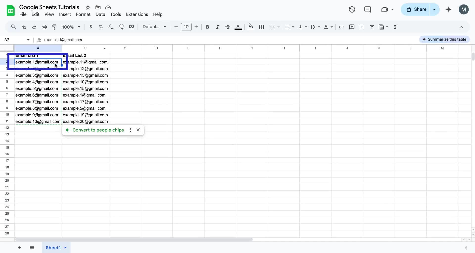
1. Select the first cell you want to start tracking the duplicates on and right-click on it to open the options menu.

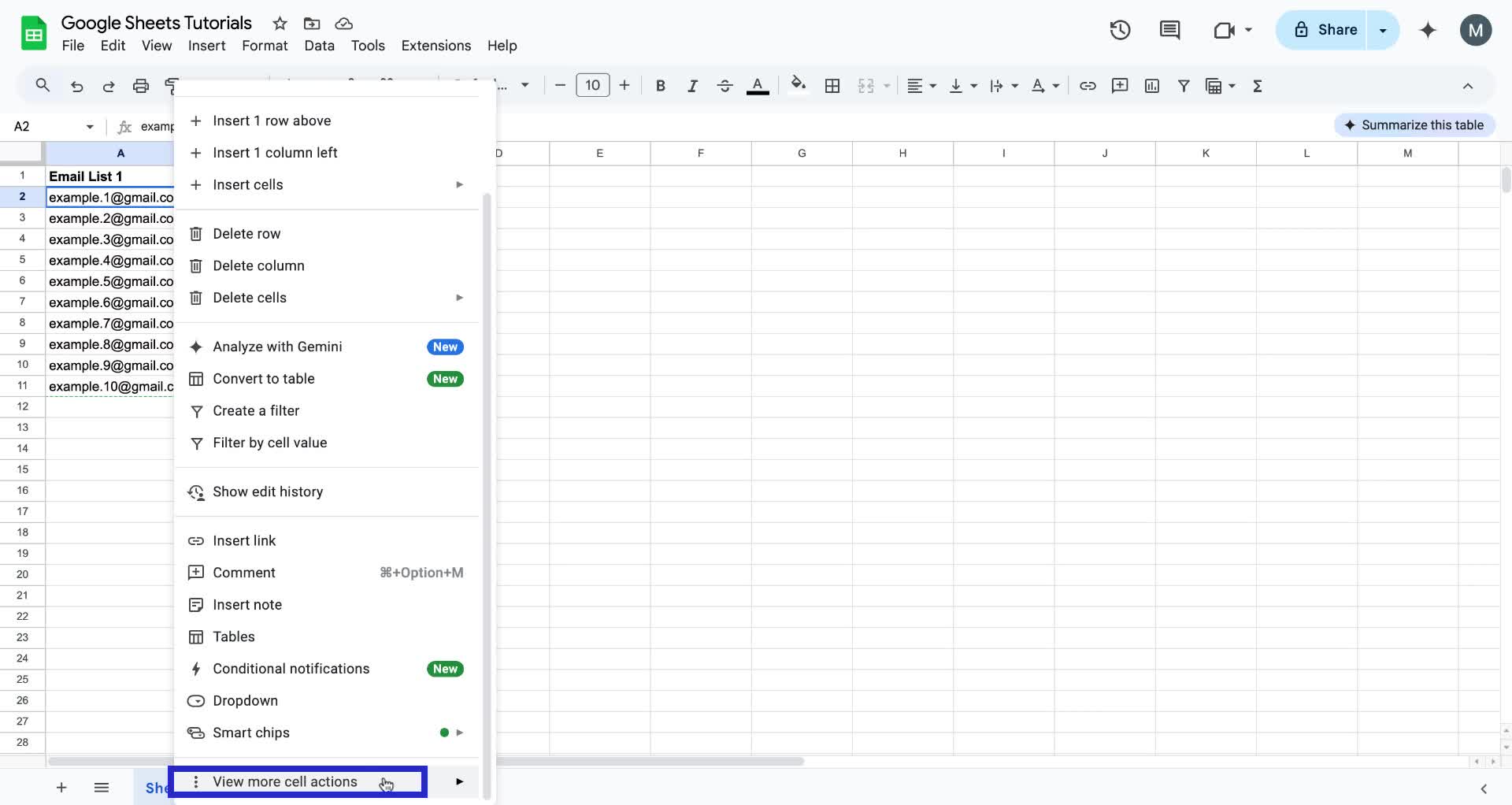
2. In the options menu, click on "View more cell actions" at the bottom.

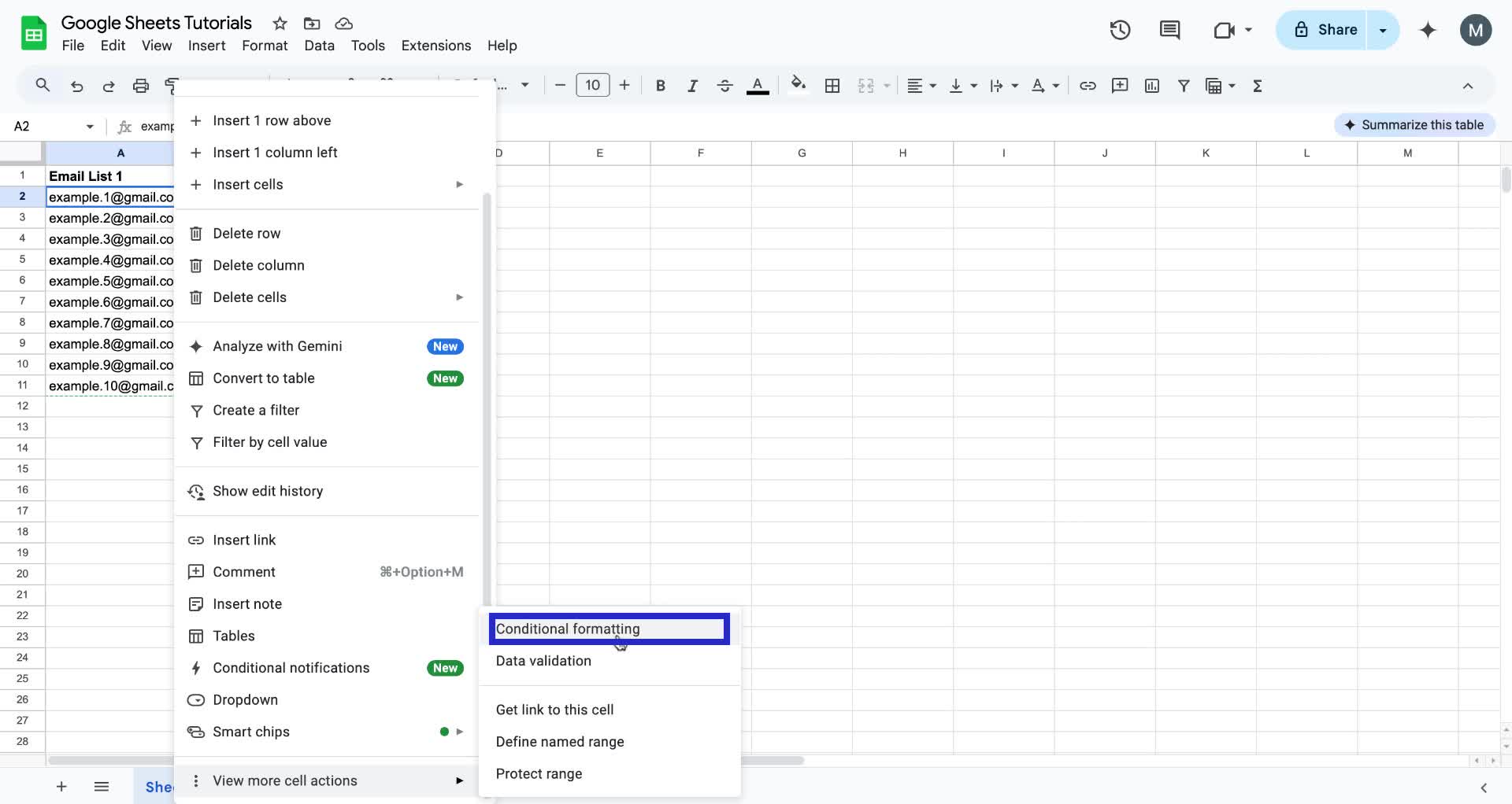
3. From the expanded menu, select "Conditional formatting."

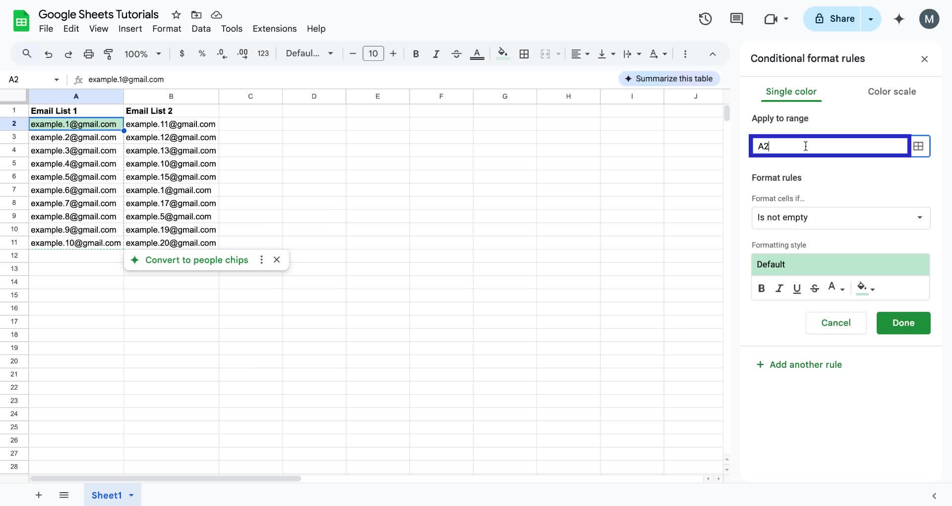
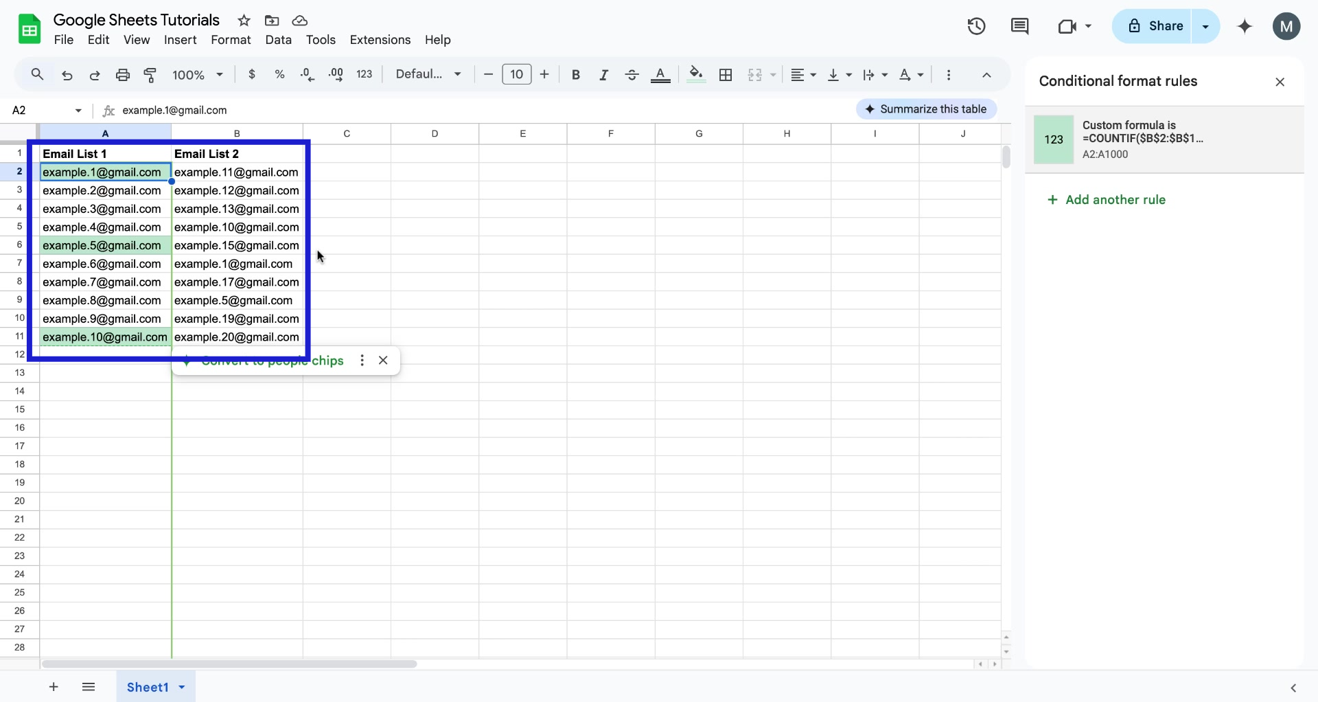
4. In the sidebar, under the "Apply to range" field, enter the value ":A1000" next to "A2". You can replace "A" with the actual letter of the column of your selected cell.

5. Then, select the dropdown menu under "Format rules".

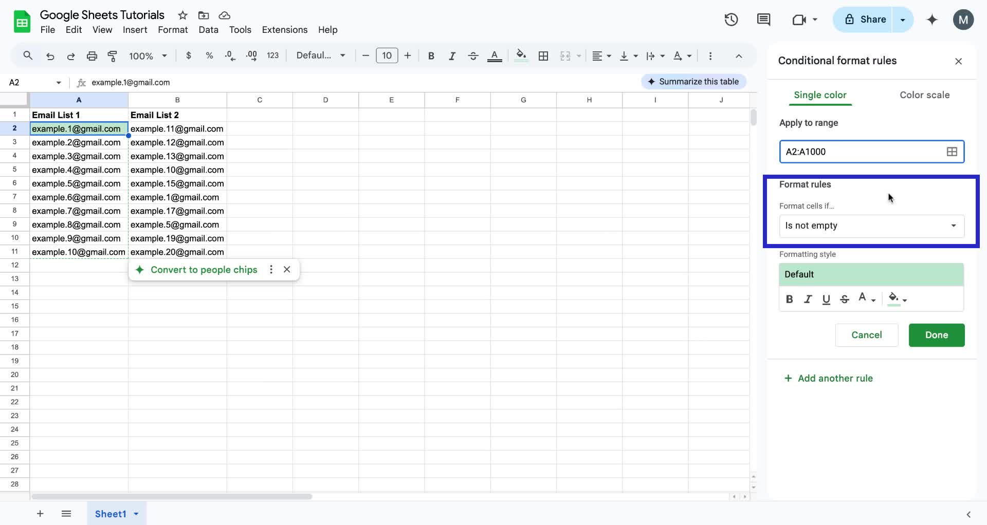
6. Scroll down the dropdown menu and select "Custom formula is".

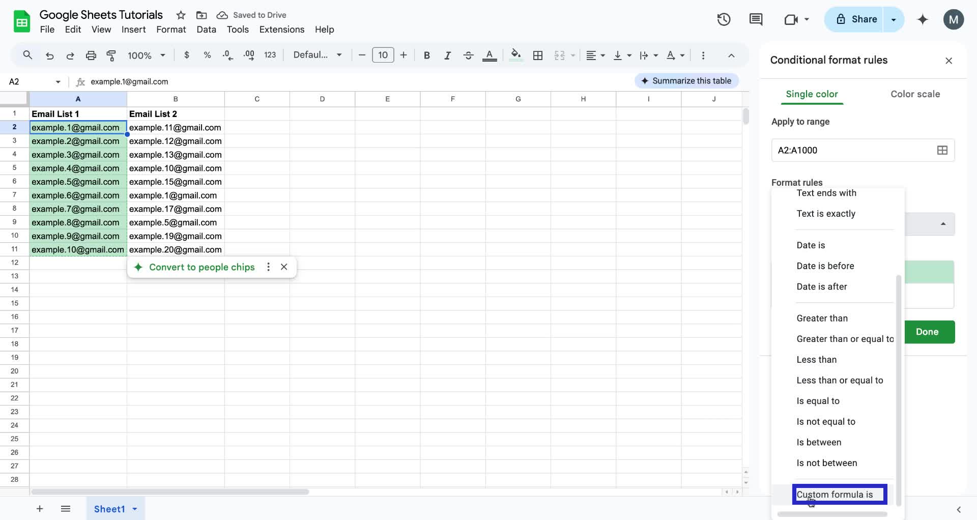
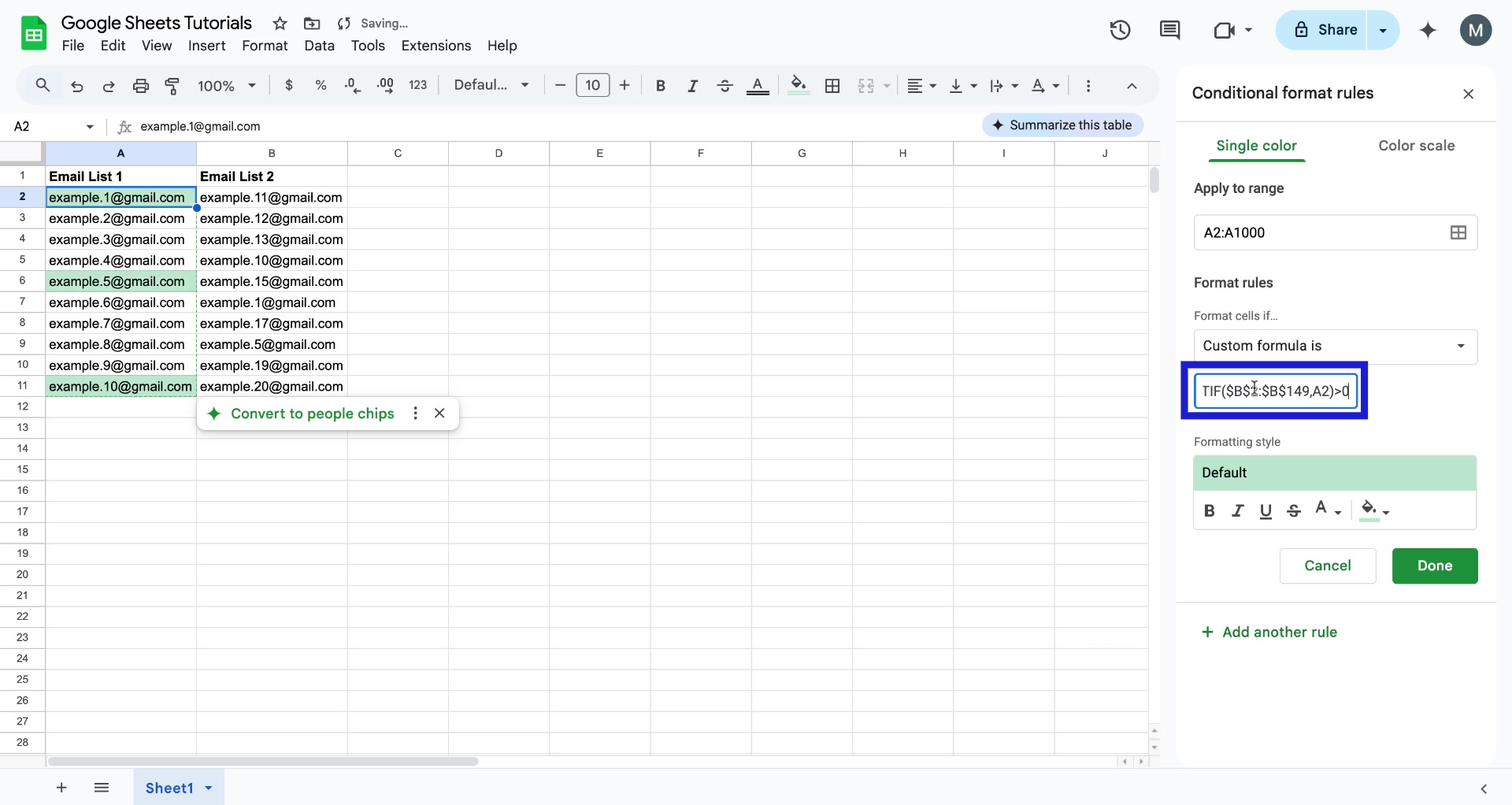
7. In the formula box, type this formula: =COUNTIF($B$2:$B$1000,A2)>0.

You can replace the letters and numbers according to the cells in your Google Sheet.

8. Then, click the "Done" button.

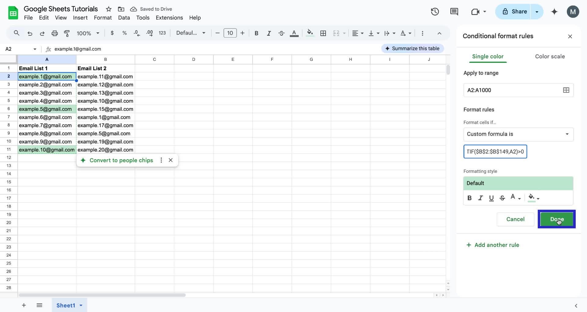
9. The duplicates are now highlighted.

Congrats! You have successfully highlighted duplicates in Google Sheets!